Far From the Shallows: Taking a Closer Look at Deep Sea Sand

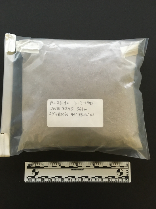
One of the great things about managing the Project MICRO SANDBOX is that one never knows what may show up at the doorstep in the form of a sand donation. Not too long ago, I received a heavy package containing nine large bags of sand with a handwritten note that read, “If this is useful, I can supply a lot more material.” Just under the note was the sand donor’s email address. Each bag of sand had a handwritten label with latitude and longitude coordinates and the depth in meters at which each sand was collected. I was intrigued, to say the least.

A quick email to my mystery sand donor put me in touch with a professor of Geology and Marine Sciences at the University of North Carolina. He explained that the samples were collected in the 1990s as part of a Ph.D. student’s research project. The focus of the research was to explain the occurrence of glauconite at various depths on the seafloor. Glauconite ((K,Na)(Fe³⁺,Al,Mg)₂(Si,Al)₄O₁₀10(OH)₂) is a greenish authigenic mineral, meaning that it is formed by crystallization where it is found, usually in marine settings commonly associated with low-oxygen conditions. The professor had sent me the sand samples not because of their glauconite content, but instead, he thought they would be of interest to science teachers because they contained large quantities of foraminifera.

Out of curiosity, I entered each of the coordinates into Google Maps, which indicated collection locations off the southern coast of Georgia. Samples collected from the ocean floor are called grabs, and for these samples, the depths ranged from 37 to 791 meters. Each grab represents only the first 5 to 10 cm of material from the ocean floor and use a box coring device: a marine geological sampling tool for soft sediments in lakes or oceans.

The professor said that using a box-coring device isn’t an ideal collection tool because box cores do not seal well, allowing some of the collected sample to be washed away during core recovery. Nevertheless, I was interested in taking a closer look at the samples. I prepared them onto sand study cards and made photomicrographs of each sample using an Olympus SZX-10 stereomicroscope.

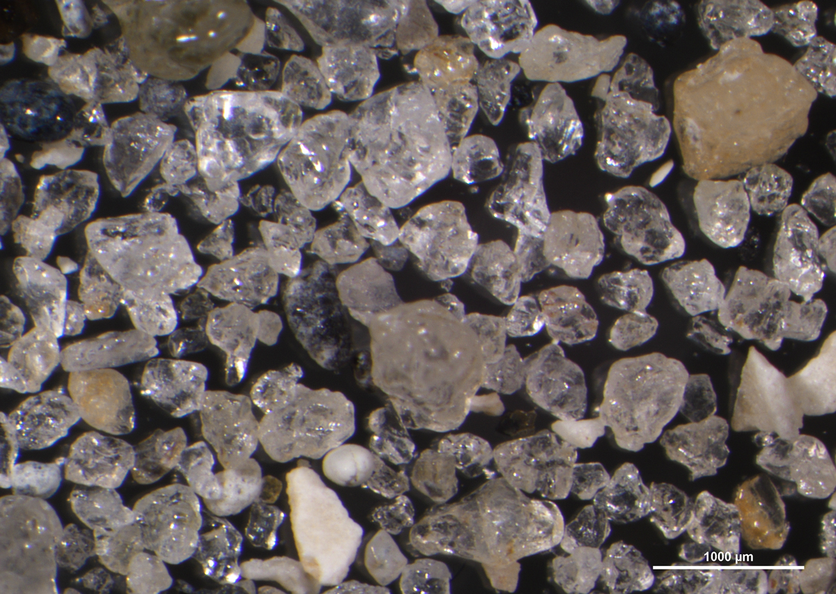
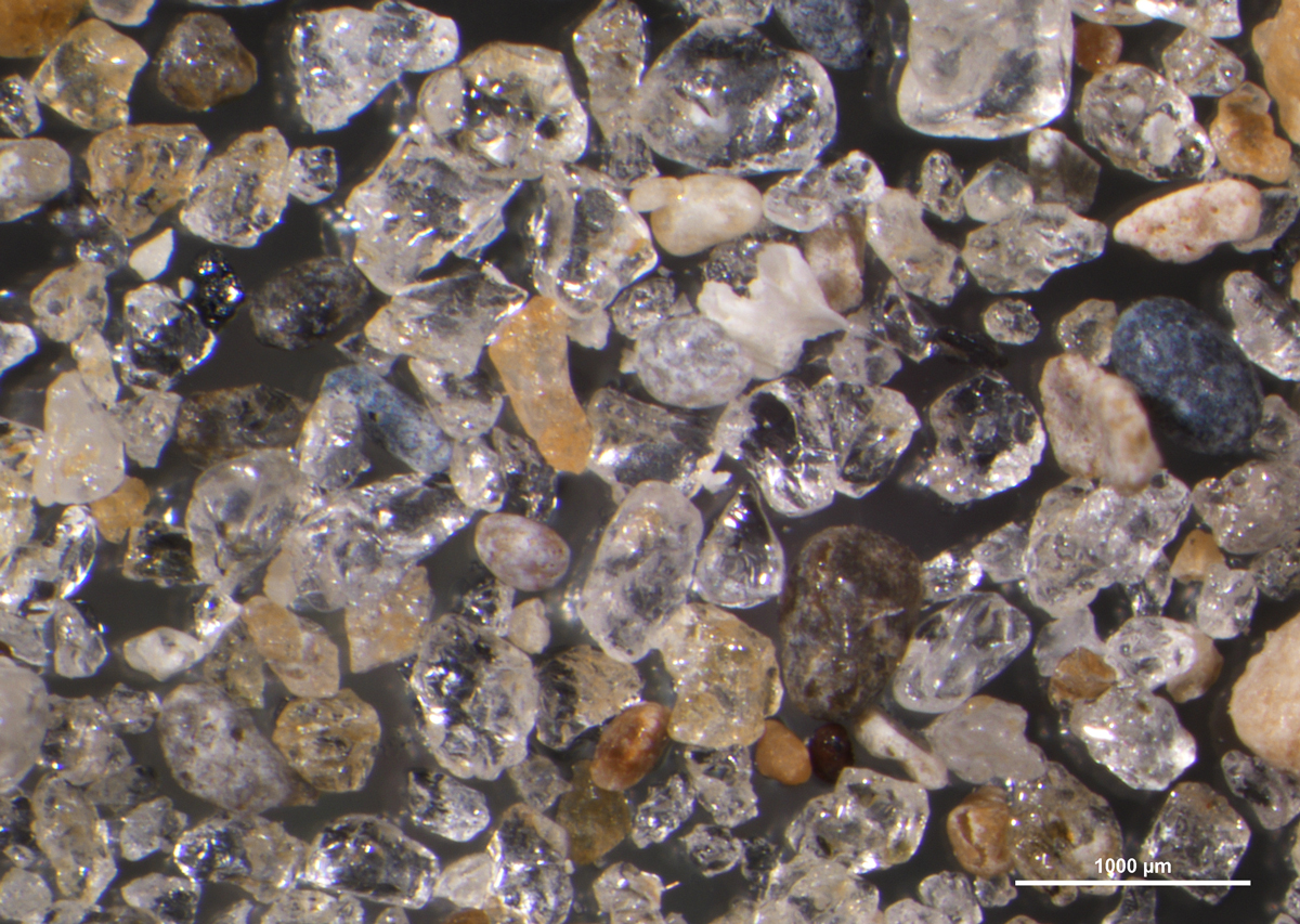
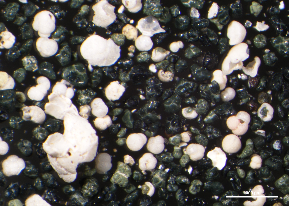
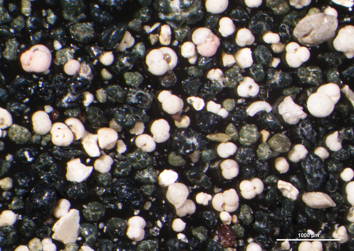
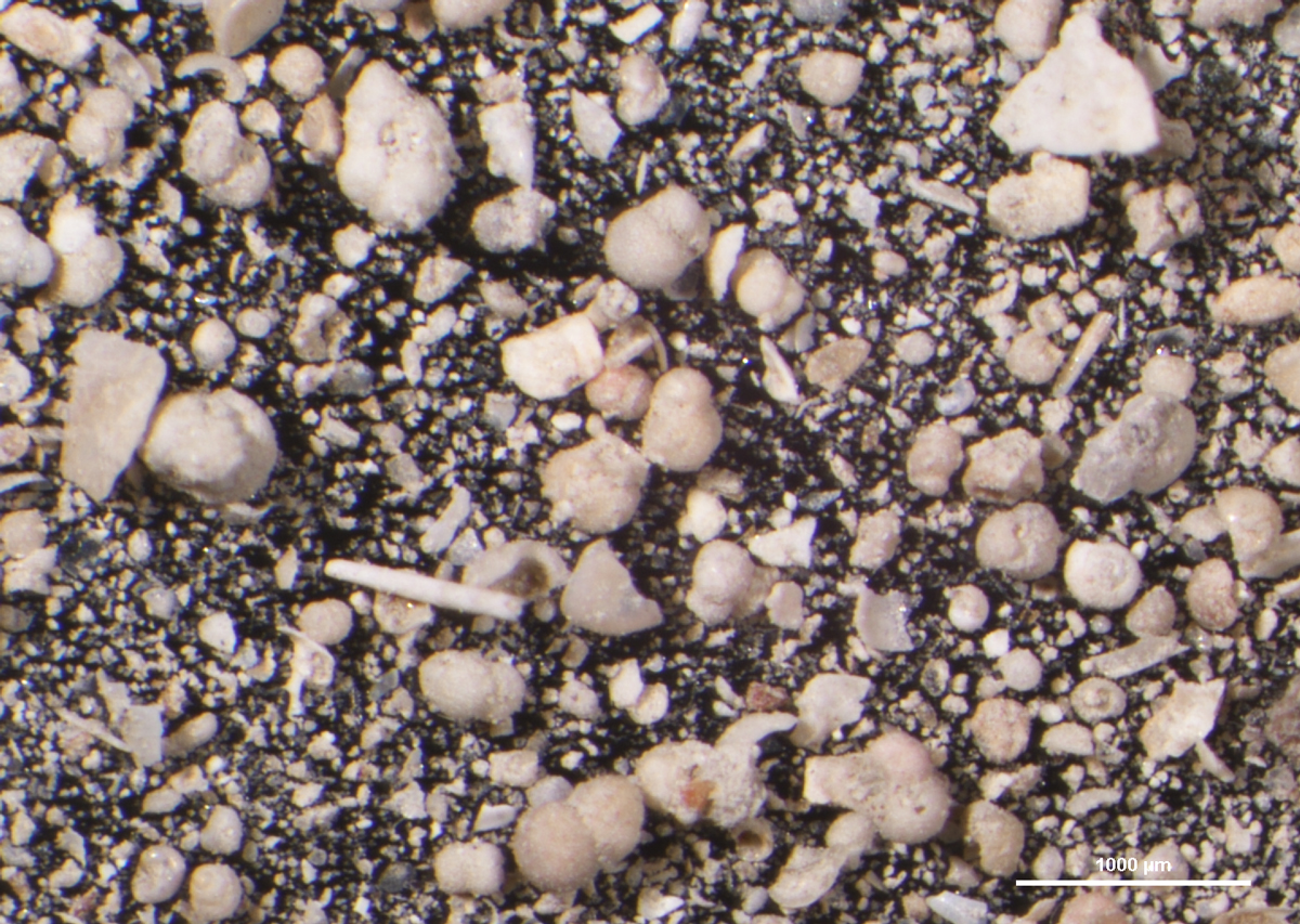
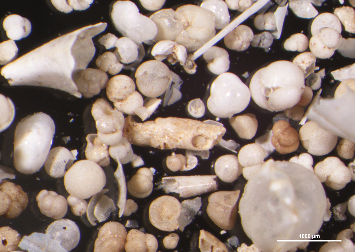
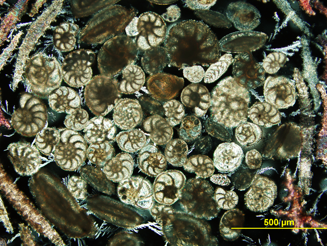
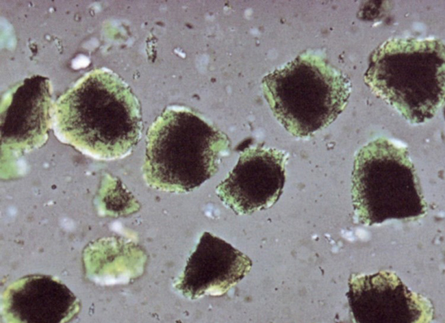
As you can see from the photomicrographs, samples collected at shallower depths—37meters and 88 meters—have no glauconite present. It is only at depths between 300 and 400 meters where we begin to see the presence of the rounded dark green particles of glauconite. This rounded shape is referred to as mamillated: covered with round mounds or lumps. As the sampling depth increases beyond 400 meters, the presence of glauconite drops off and significant quantities of foraminifera begin to appear.

Glauconite was first described in 1856 by J.W. Bailey while looking at material collected from the ocean floor off the Atlantic coast near New Jersey. Bailey refers to glauconite as “greensand” and he also noted that “…mineral matters diminish with increased depth while organic remains increase.” Bailey’s observations are consistent with the deep sea sand samples pictured above.

An Ocean-sized Endeavor

The most comprehensive study of deep sea sand was carried out over a four-year period from 1873 – 1876 on board the HMS Challenger, which set sail under the command of Captain George S. Nares, with the scientific undertaking of investigating the world’s seafloors. The study took four years to complete and employed two techniques: sounding and dredging. Sounding measures the depth of the ocean, while dredging brings collected material up to the surface for analysis.

To pull off such a huge undertaking, the ship employed a crew of 292, including a handful of natural scientists referred to as “Scientifics.” The chief scientist among them was Wyville Thomson who oversaw the sounding and dredging activities and the ship’s well-equipped lab, which included several microscopes.

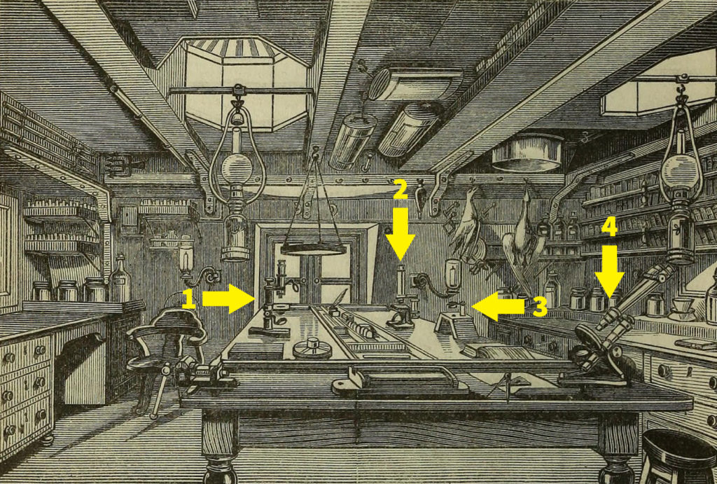
The image above gives you a sense of what the Challenger’s laboratory space looked like and the equipment frequently used. You can see that there are several microscopes available in the laboratory to characterize and describe the contents recovered from the ocean floor. In the book The Voyage of H.M.S. Challenger 1873-1876: Deep-Sea Deposits, written by John Murray, one of the Scientifics on the ship talks about the microscopical observations of recovered glauconite:

• “The most typical glauconite sands of the Challenger collection contain 40 to 50 percent of foraminiferous and other carbonate of lime shells together with remains of silicious organisms.”
• “The individual grains of glauconite that occur in marine deposits rarely if ever exceed 1 mm in diameter.”
• “The typical grains are always rounded, often mamillated, hard, black, or dark green…”
• “They have occasionally the vague form and appearance of foraminifera and other organisms…”

In addition to Murray’s glauconite descriptions, I was curious to know more about the microscopes pictured above. In the same book, Murray describes his use of two of the microscopes:

“The microscopes used most frequently by Mr. Murray were a Ross binocular with low powers and a Hartnack with high powers; these were firmly clamped to a small table, fixed securely into the deck of the ship.” (I added yellow arrows and numbered each of the microscopes for discussion purposes.)

• Microscope #1 is the Hartnack
• Microscope #2 may be a Hartnack also; it has the same horseshoe base as Microscope #1
• Microscope #3 is a single lens mounted to a wooden platform for low power gross observations
• The Ross microscope is labeled #4

With this bit of information in hand, I consulted The McCrone Group’s onsite Brooks Collection of Antique Microscopes to see if I could find anything related to this historic voyage. I found:

• Ross binocular microscopes, but none having the same configuration as the one pictured
• Books describing the evolution of Hartnack microscope designs
• A curious nickel-plated microscope built by Constant Vérick, an apprentice of Hartnack’s
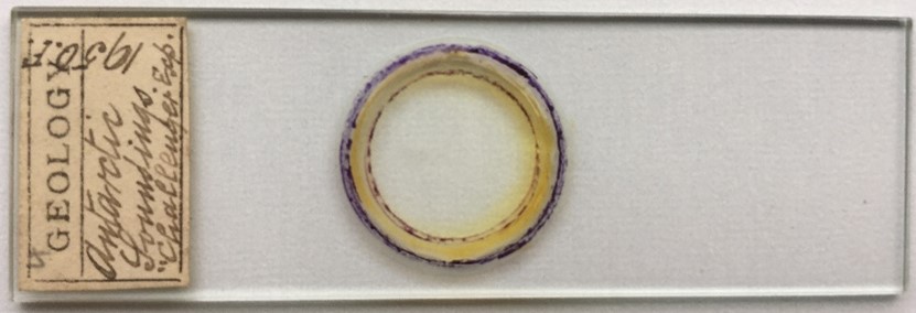
• A microscope slide preparation from the Challenger Expedition

Let’s start with Hartnack and his microscopes.

The Sincerest Form of Flattery

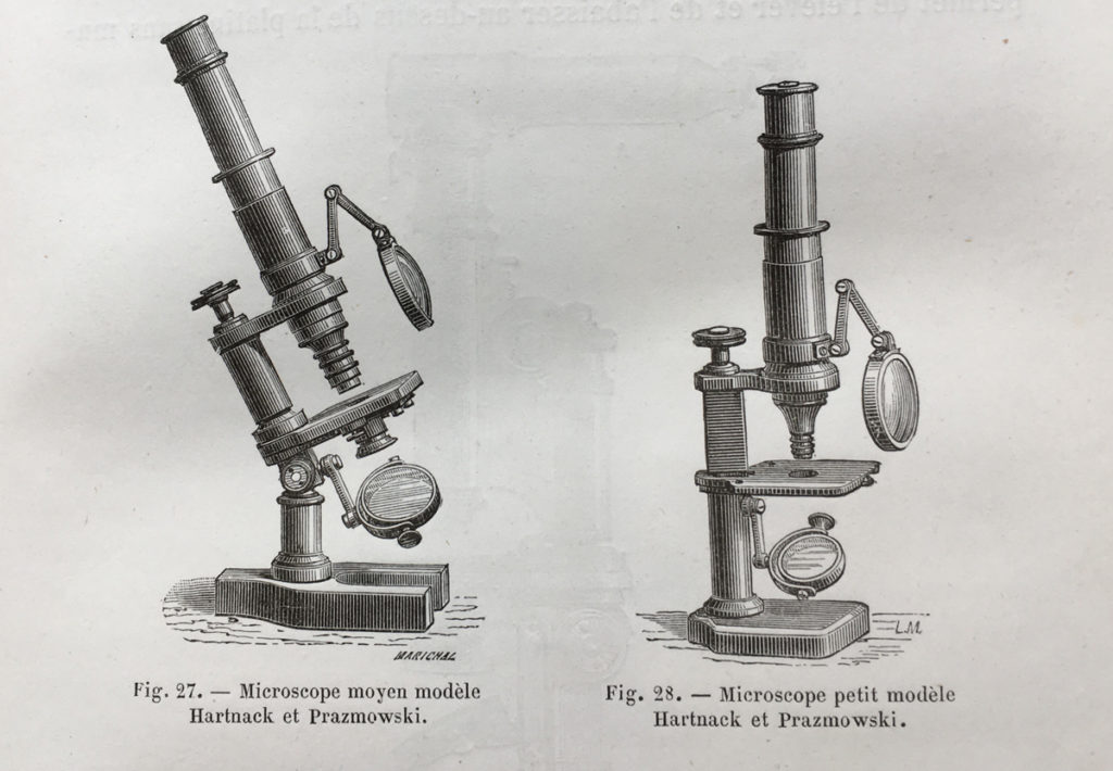
Like many microscope designers of the past, the Hartnack microscope follows a lineage starting with Georg Oberhäuser. Oberhäuser was an instrument maker in Paris in the 1830s who eventually partnered with his assistant, Edmund Hartnack. Shortly after forming this partnership, Oberhäuser retired and Hartnack took over the business. Hartnack eventually employed an apprentice by the name of Marie Constant Vérick for several years, who went on to form his own instrument company in the early 1870s. Later, Hartnack partnered with Adam Prażmowski, whose name is referenced under the microscopes in the woodcut below. For a more thorough historical treatment of the Hartnack microscope, I recommend you check out Brian Stevenson’s articles.

Since I couldn’t get my hands on a Hartnack microscope, I focused my attention on the nickel-plated Vérick microscope—it’s what I would call a Hartnack knockoff, which Vérick freely admits, sort of.

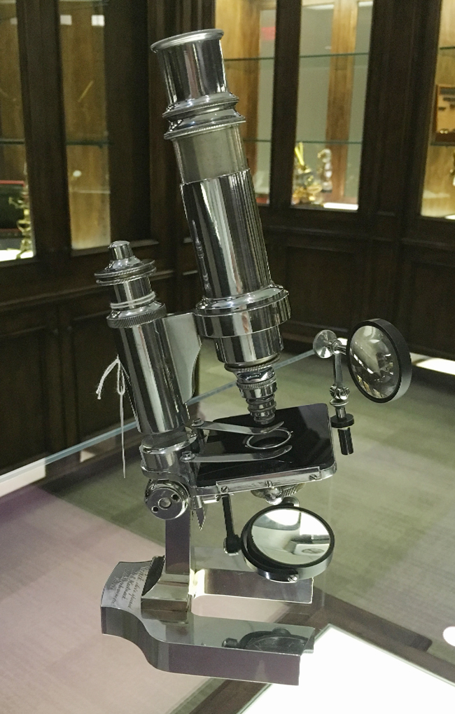
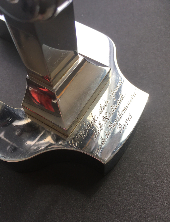
Comparing the drawings of the Harnack microscope to the nickel-plated Vérick pictured above, you can see that the Vérick is pretty much an exact copy of the Hartnack. It was common for microscopes made during this era to have engraved somewhere on the microscope’s base, the designer of the instrument and the address of the shop. Perhaps to bring the Hartnack microscope reputation (and design) with him, Vérick would inscribe “C. Vérick élève spécial de E. Hartnack, rue de la Parcheminerie 2, Paris” on the base of his microscopes. The words “élève special” translate from French to English as “special student”, a title that Vérick bestowed upon himself.

History Under a Cover Glass

The most interesting find in the Brooks Collection was a microscope slide preparation from the Challenger Expedition. As I held the preparation in my hand, I couldn’t help but wonder who made the slide? Maybe John Murray or Wyville Thomson himself? The slide label indicates the sample was collected during the Antarctic soundings at a depth of 1,596 fathoms (3577 meters). One of the Scientifics probably examined the slide with the Hartnack microscope, under calm conditions, while docked in some far-off harbor.

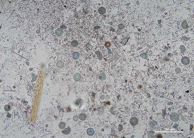
Placing the preparation under an Olympus BX51 microscope revealed a strew of diatoms along with what looked like a piece of plant material.

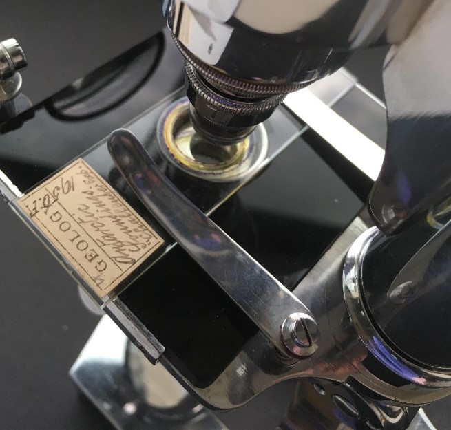
While I was satisfied with my images from the Olympus microscope, I couldn’t resist the temptation to examine this prep using the Vérick. This would be my closest attempt to recreate what the Scientifics might have experienced aboard the Challenger.

Setting up the microscope was a bit of challenge. The focusing mechanism is a knurled ring that sits atop the vertical pillar just behind the monocular observation tube. Turning the knob raises and lowers the monocular observation tube. The objectives are designed to nest within each other and come apart by unscrewing them. I removed the highest magnification lens revealing a moderate magnification, maybe a 20X lens. I also gave the microscope a general dusting and used Scotch^® tape to clean the eyepiece and the mirror below the stage. The optics could use a better cleaning, but since this was a valuable antique, I thought it best to keep that kind of thing to a minimum.

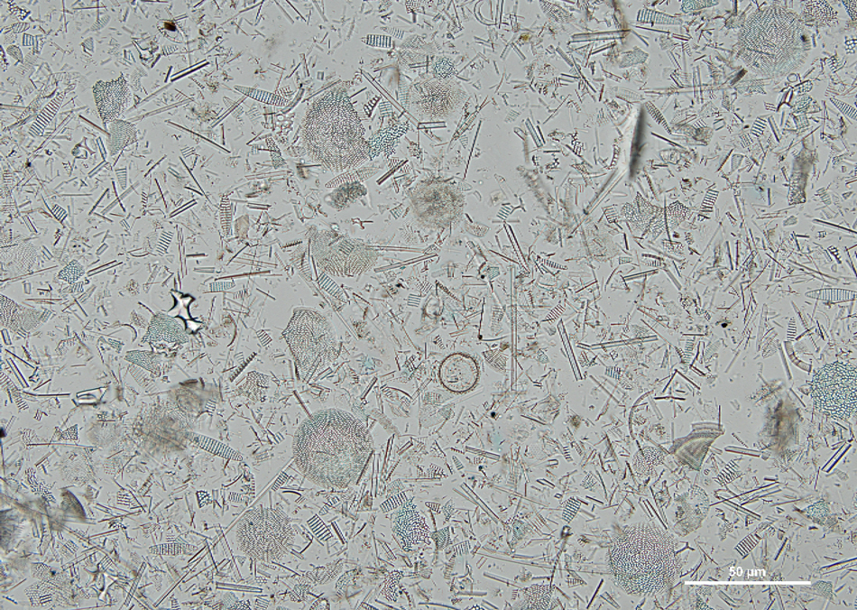
I placed the Challenger slide on the Vérick stage and turned the mirror toward the cloudy sky. The image slowly came into focus after much turning of the focusing knob. What I saw was a somewhat milky image. Holding my smart phone camera just above the eyepiece, I tried to capture a similar field of view as the BX51 image for comparison. I thought the image quality wasn’t too bad for an instrument that was nearly 150 years old.

Hiding In Plain Sight

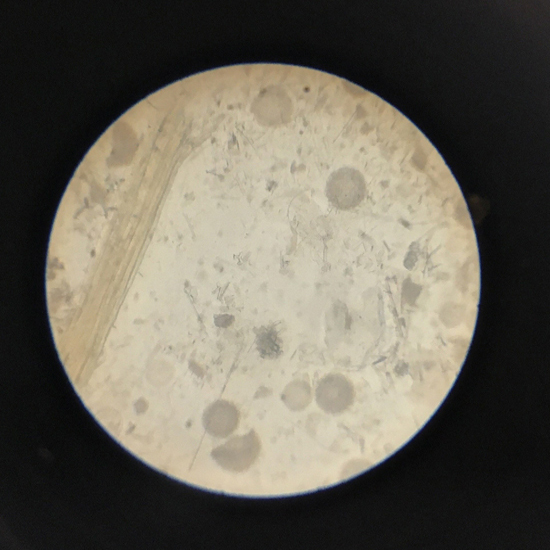
As I came to end of this curious trail that began with the mystery sand donation, I wondered if the sample of foraminifera used in our polarized light microscopy course might contain glauconite. I grabbed a 100-particle reference set and plucked out Slide #4—Foraminifera.

I have examined this sample before over the years, but this time I was looking for any evidence of Bailey’s “greensand”. I first scanned the slide using transmitted light and noticed several dark green, almost opaque grains mixed in with the foraminifera. I switched my lighting conditions to reflected light, in the hopes of getting a better rendering of the true color of these grains. There did appear to be a small amount of glauconite in our foraminifera reference sample.

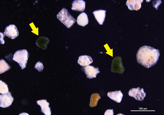
The suspected glauconite grains in this preparation seemed to lack the textbook mamillated morphology, but perhaps our reference sample was collected at a shallower depth, and therefore the conditions were less than optimal for the glauconite to fully form? Some of this may be speculation on my part, but whatever the case may be, I now have a deeper appreciation to be on the lookout for glauconite when examining foraminifera.

For a more thorough microscopical characterization of glauconite, check out the following references.

• McCrone, W.C.; Delly, J.G.; and Palenik, S.J. (1973). The Particle Atlas, Edition Two, Volume III, Ann Arbor Science Publishing Inc. #149 Glauconite, slightly uncrossed polars:

“The rounded, fine-grained aggregates of this hydrous silicate of iron and potassium constitute a sedimentary marine deposit usually associated with clays and sand. It consists of minute, overlapping, transparent platelets; some single crystal grains are roughly hexagonal in outline. The fine laminae show a distinct micaceous cleavage. The color is green, olive green or blackish green (011010); particles less than 2 µ diameter are colorless (001010). Higher iron content causes a shift toward red and higher refractive indices. The indices of this monoclinic, biaxial mineral are 1.590-1.612 (α), 1.609-1.643 (β), 1.610-1.644 (γ); (-) 0.014-0.032; 2V = 0°-20°, but usually greater than 10°. Specific gravity ranges from 2.4 to 2.95; hardness is 2. Individual crystals are strongly pleochroic with α pale to straw yellow, β and γ green, dark green, bluish green or olive green. The yellowish and brown particles in the photomicrograph are limonite and geothite, alteration products of glauconite.”

• Winchell, A.N. and Winchell, H. (1951). Elements of Optical Minerology: An Introduction to Microscopic Petrography, pp. 377-378.
• Deer, W.A., Howie, R.A., Zussman, J. (1995). The Rock Forming Minerals, 2nd Edition, p.296.
• Nesse, W.D., (2004). Introduction to Optical Minerology, 3rd Edition, 174.