How to Make and Use a Simple Microspectroscopic Eyepiece

INTRODUCTION

Here’s a fascinating and highly useful accessory for your microscope, which you can make for less than one U.S. dollar. The simple microspectroscopic eyepiece described is suitable for most qualitative work, and even some semi-quantitative analyses. Let me first tell you how to make your own microspectroscopic eyepiece, and then I’ll tell you how to use it and experiment with it. I first wrote about this device in 1966 (1), when inexpensive, acetate plastic diffraction grating replicas having about 13,400 lines per inch first became commonly available. Since that time, holographic diffraction grating replicas have become available at very reasonable cost, allowing for improvements in performance, with no increase in cost.

First of all, you will need an eyepiece with a focusing eyelens—the kind that you probably already have for your eyepiece micrometer. It can be an older model with focusing accomplished by sliding the telescopic tubing up and down, or it can be a more modern eyepiece with helical focusing of the eyelens. Remove the graticule from the eyepiece in preparation for the modification. The microspectroscopic eyepiece consists only of a slit, and a piece of diffraction grating replica film. Refer to Figure 1, a cross section of an eyepiece with focusing eyelens, for placement of the parts.

ASSEMBLING THE SIMPLE MICROSPECTROSCOPIC EYEPIECE

The Slit: The slit is made from a double-edge razor blade, and a piece of cardboard or a washer. Cut a round piece of thin cardboard so that it will lie on the eyepiece diaphragm, or on the eyepiece graticule mounting shelf. A U.S. 5¢ piece or an English sixpence coin makes a perfect template of correct size for diaphragms of older eyepieces. Cut a rectangular opening in the disc—see Figure 1. There is nothing critical about the dimensions of the cut-out, for it only acts to support the razor blade pieces.

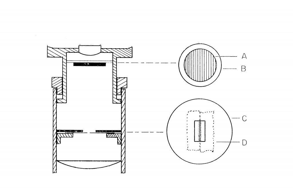
Next, snap a double-edge razor in two, using a couple of hemostats or long-nosed pliers—and don’t forget to wear eye protection; a tin snips works even better. Then, snap one of the long halves in two, put the two cutting edges face-to-face to form a narrow slit—say, about 0.2 mm to begin with, and tape or glue them to the cardboard (I used double-sided sticky tape). See “D” in Figure 1 for placement of the razor blades on cardboard disc, “C.” You might want to make a couple of these slit assemblies, with different slit widths. The narrower the slit, the greater will be the spectral line resolution, but the less light there will be, necessitating a higher wattage lamp.

Place the slit blade-side-down on the diaphragm of the eyepiece. You can paint everything flat black, if you want to, but if you use “blued” blades, this will not be necessary. I have been having trouble finding blued blades recently, so, for my most recent version, I used the more commonly available stainless steel blades. I used a pair of tin snips to cut them to size, and trim them.

Figure 2 shows all of the parts that you will need to convert any eyepiece with a focusing eyelens, including washers, razor blade, flat-black paint, and gun blue; a completed razor blade slit mounted on a blackened washer is also shown in place on the graticule mounting shelf of an Olympus eyepiece. For the Olympus BX-51 polarizing microscope I am currently using, a WHI0X-H/22 high-eyepoint eyepiece was converted. The graticule size for this eyepiece is 24 mm. I looked in my baby food jar of miscellaneous washers for one of that size and the closest I found was 1-inch diameter. I turned this down to 24 mm in my miniature lathe. Incidentally, a U.S. quarter (25¢ piece) is just over 24 mm (24.12 mm-24.25 mm), so it makes a good template for a cardboard disc.

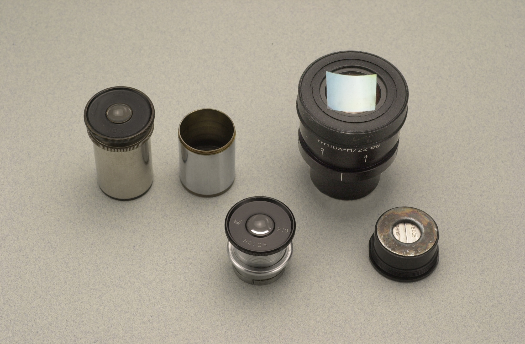
Figure 3 shows a couple of older eyepieces with focusing eyelenses, together with the new Olympus WH10X eyepiece. The eyepiece at the far left has been reassembled; in the middle, the focusing eyelens has been removed to gain access to the diaphragm; at the far right is the Olympus WH10X-H/22 eyepiece with a piece of holographic diffraction grating replica sitting on top of the eyelens, and in front of it, the slit is shown before being screwed back in the base of the eyepiece.

It is not necessary to darken the washer and blades, but blackening them does cut down on internal glare. You will have to expose fresh, clean steel for the gun blue to “take.” The gun blue I prefer consists of selenious acid, hydrochloric acid, and copper sulfate. I also use Kodak Dull Black Brushing Lacquer, but any flat black paint will do.

Diffraction Grating: Inexpensive transmission diffraction grating replicas are what makes all this possible; there are two kinds, ruled and holographic.

Ruled diffraction gratings are produced by ruling a closely-spaced series of straight, parallel grooves into an optically-flat, aluminum-coated substrate, using an interferometrically-controlled ruling engine to guide a diamond cutting tool. The diamond tool forms a sawtooth-shaped groove profile at a specific angle known as the “blaze” angle. The finished, ruled grating is known as the “master” grating. Replicas are made from the master by vacuum deposition coating the master with a separation layer, and then aluminum coating the top of the separation layer. For commercial gratings, an epoxy-coated flat-glass substrate is placed on top of the layer-covered master, thus duplicating the grooved surface. The combination is cured, and the replica is separated from the master. Such commercial diffraction grating replicas range in cost from about $65 to $200, depending on size and number of grooves per millimeter. Fortunately, very inexpensive non-commercial grade diffraction grating film is available. Forty years ago, I used a film that had 13,400 lines per inch. I bought it from American Science Center in Chicago; a 2” X 2” piece cost 25¢, and a sheet 8/2” X 11” cost $1.50. This is no longer available. However, Edmund Scientific’s Scientifics® (www.scientificsonline.com) sell a diffraction grating film with 1,000 lines per millimeter; two sheets 12” X 6”, catalog #E30402-67, cost only $7.95. They also sell 2” X 2” cardboard-slide-mounted diffraction grating film with 13,400 grooves per inch, catalog #E30073-07; a package of 15 costs $7.95.

Holographic gratings are formed from laser-produced masters. Two laser beams form an interference fringe field, whose standing wave pattern is exposed to a photo-resist coated polished substrate. The resulting pattern of straight lines has a sinusoidal cross section. Replicas are made in a manner similar to that for ruled gratings. Holographic diffraction gratings have a decreased amount of stray light, and, therefore, produce sharper diffraction orders than ruled gratings, which, in turn, increase the ability to view spectral absorption and emission lines by placing most of the light in the first-order image. Commercial-grade, holographically-produced gratings range from $75 to $300, depending on the size and number of grooves per millimeter. Again, inexpensive, non-commercial grades are available. Scientifics sell a holographic diffraction grating film made from 0.002” thick, clear polyacetate film with 12,700 grooves per inch. A set of two sheets 12” X 6”, catalog #E30545-09, costs $7.95—same cost as the ruled film. Or, a package of 15 cardboard-slide-mounted gratings, catalog #E30545-10, costs $9.95.

Another source for holographic diffraction grating replica film is Learning Technologies, Inc. (Project STAR), 1-800-537-8703. Their film has 19,050 lines per inch (750 lines per millimeter), with a dispersion angle of 23.5°. The replica is made of polyester plastic, and they claim their material is 100 times more efficient than acetate gratings. Two 5” X 5” sheets, catalog #PS-08-A, cost $9.00. It is also available as a 6′ X 5” roll, 4.5” X 5” sheet, and even as a single 35 mm glass slide.

Contact McCrone Microscopes & Accessories about these diffraction gratings.

Cut a circular or square piece of diffraction grating replica film, “A” in Figure 1, and insert it directly beneath the eyelens, supporting it there with a wire retainer, or “O” ring, or cork ring; or, you can fix it to a cover glass, being careful not to cement the ruled side of the grating. For the newer Olympus eyepiece, I cut a 1/2;” X 1/2” diffraction grating film and placed it right on top of the eyelens (Figure 3); this is faster, and it works just fine. How do you know which way the rules/grooves are running on your film? Look at the film with your microscope, using at least a 40X objective. Compare the ruled diffraction grating to the holographic grating; and, equally interesting, compare the holographic gratings from Scientifics and from Learning Technologies. Eventually, you will want the rulings to be correctly oriented with respect to the slit—rulings parallel to the slit.

SET-UP OF THE SIMPLE MICROSPECTROSCOPIC EYEPIECE

The simple microspectroscopic eyepiece is now completed. Insert the modified eyepiece into the microscope, turn on the light, and adjust the eyelens until the slit is in sharp focus for you. It will be easier now if you replace the other, unmodified eyepiece with a dust plug. Now look to the far left and far right of the slit; the continuous spectrum of the light source will be seen on either side of the slit. Look still farther, left and right, beyond these first-order spectra, and you will see another set of spectra, more expanded (dispersed), but less bright beyond the brighter spectra; these are the second-order spectra. The slit may be positioned to one side of center, so that the spectrum will be centered. Try both ways. Also, one of the spectra may be sharper than the other one. Rotate the diffraction grating film that is sitting on top of your eyelens, and notice that, if the rulings/grooves are perpendicular to the slit, you will see images of the slit above and below the actual slit, but only when the film is rotated so that the rulings/grooves are parallel to the slit will you obtain nice spectra to the left and right of the slit. If there is dirt in the slit, or any dust particles adhering to the razor blade edges, thin black horizontal lines will be seen running across the spectrum.

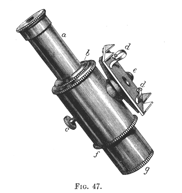
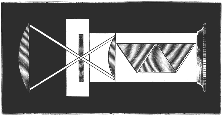
Tilt your mirror, if you have one, toward a fluorescent light, and the mercury spectrum will be seen superimposed on the entire visible spectrum. You will see stronger lines in the yellow, green, and blue. See if you can resolve the two yellow lines at 577 nm and 579 nm. The green line will be at 546 nm, and the blue line lies at 436 nm. Without a scale in the field-of-view, only qualitative work can be done, but this is sufficient for most purposes. The microspectroscope made by Zeiss about 70 years ago, like the original Sorby-Browning, utilizes a direct vision prism, and has not only an illuminated, adjustable scale, but a right-angle prism and side port for introducing a reference spectrum that can be seen simultaneously with the spectrum of the substance under investigation. You can read about the Zeiss Microspectroscope in Needham’s The Practical Use of the Microscope (2). Figure 4 is a woodcut of the original Sorby-Browning Microspectroscope of the 1860s and Figure 5 is a woodcut of the cross section of this device.

All right, now we have a caution for all of you who are trying this with a polarizing microscope. If you leave your polarizer in, you will get all kinds of strange anomalies when you look at a spectrum of your light source (note what happens to the appearance of your spectrum as you rotate the polarizer). So, you need to remove the polarizer. This will be easy with many microscopes; however, the polarizer is not removable from the condenser of the Olympus microscope. At this point, you can modify the Olympus pol condenser so that the polarizer is removable (see my article, reference 3, on the simple steps to do this), or you can change the condenser to a non-pol—I changed to an achromatic aplanatic 1.4 NA non-pol condenser.

If your microscope does not have a mirror, but only a fixed light-exit port, it is worth making an attachable mirror by cutting a metal disc to the size of your light-exit port, and drilling a hole in the middle to take the adjustable mirror in its fork mount from any commonly available microscope that does not have built-in illumination. The attachable accessory mirror made by Zeiss, shown in Figure 6, will serve as a model.

One other point, before we leave the set-up of the microspectroscopic eyepiece, and get into its application: after you have gotten the slit in focus, and have the rulings/grooves running parallel to the slit, as evidenced by the observable spectra to the left and right of the slit, darken the room, remove any filters, neutral densities, etc. from the light path, direct all of the light to come out of the inclined tubes by proper prism selection, put an eyetube plug in the place of the unmodified eyepiece if you haven’t already done so, and hold a thin 3” X 5” piece of white paper a couple of inches above the microspectroscopic eyepiece. You will see projected on this paper screen an image of the slit, and both sets of first-order and second-order spectra. This is convenient for demonstration and group discussion.

WHAT TO LOOK AT

Now that you have a completed and tested microspectroscopic eyepiece, what do you look at? The answer is, anything that is colored, and even some colorless or nearly colorless substances with strong absorption in select regions of the spectrum. You can look at colored lights, or solids, or liquids. Seeing the mercury lines from a fluorescent lamp superimposed on a complete spectrum suggests that you could view the light from sodium vapor lamps, or cadmium or neon; or street lights of various kinds and colors. These are emission spectra.

Emission spectra can be produced by spark vaporizing the material under test, and looking at the light thus produced. Flame tests are a common form of flame emission, in which a platinum wire is dipped into a solution or salt of, say, sodium, or potassium, or strontium, or copper, or calcium, and then placed in a Bunsen or alcohol lamp flame. The flame will be colored. Mixtures of such salts are sold for placing on logs in a fireplace to achieve novel, colored flame effects. If these colored flames are viewed in a spectroscope—or with your microspectroscopic eyepiece—the background will be black, but a series of colored lines will be seen that are characteristic of the metal element. The exact wavelengths of these colored lines have been well documented over time, and form the basis of emission spectroscopic analysis. The characteristic lines of each element, and their intensities, may be found in any edition of The Handbook of Chemistry and Physics, or in the several editions of the classic textbooks on spectrum analysis, such as those by Roscoe (4), Lockyer (5), or Schellen (6). The more complete M.I.T. Tables of Wavelengths are not needed for our purposes.

An absorption spectrum occurs when light passes through a cold, dilute gas and atoms in the gas absorb at characteristic frequencies, or when any colored substance is introduced between the light source and the spectroscope. Absorption spectra are characterized by a continuous spectrum displaying periodic, vertical black lines or bands of varying intensity and width. Interposing colored filters or substances between the light source and the microspectroscopic eyepiece will result in absorption spectra.

Figure 7 illustrates the solar spectrum with its absorption lines, and the emission spectra of the metals of the alkalis and alkaline earths. This color plate is the frontispiece of Roscoe’s book (4) on spectrum analysis. Figure 8 is another chromolithographic plate from his book, showing the spectra of some of the stars and nebulae. Roscoe was an English chemist who, after his undergraduate work, trained with Bunsen at Heidleberg for his Ph.D. in 1855. He translated Bunsen and Kirchhoff’s classic, Chemische Analyse durch Spectralbeobachtungen (1860), and Kirchhoff’s Untersuchungen Über das Sonnenspectrum (1861-63), and includes a number of their tables and spectra in his own book.

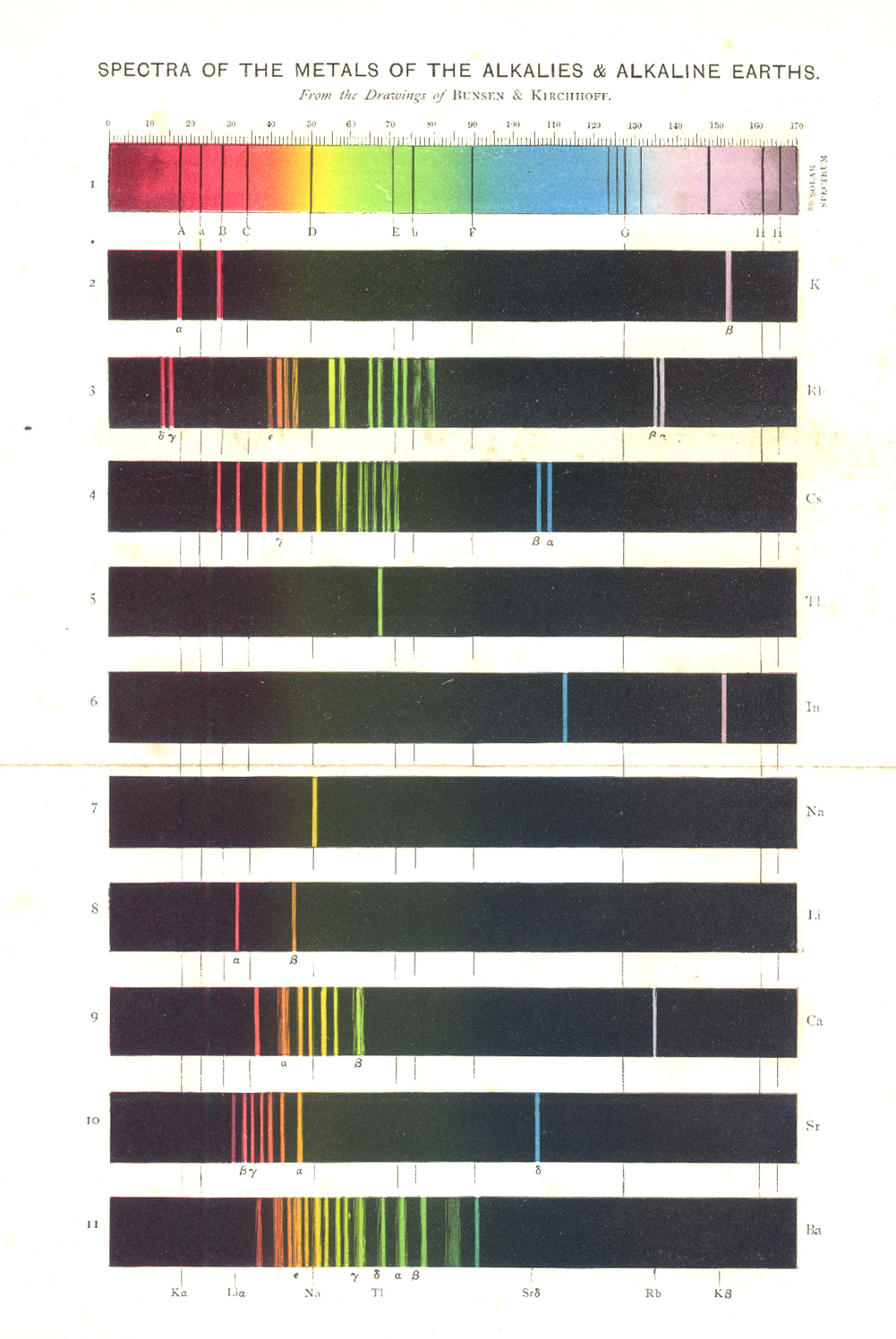
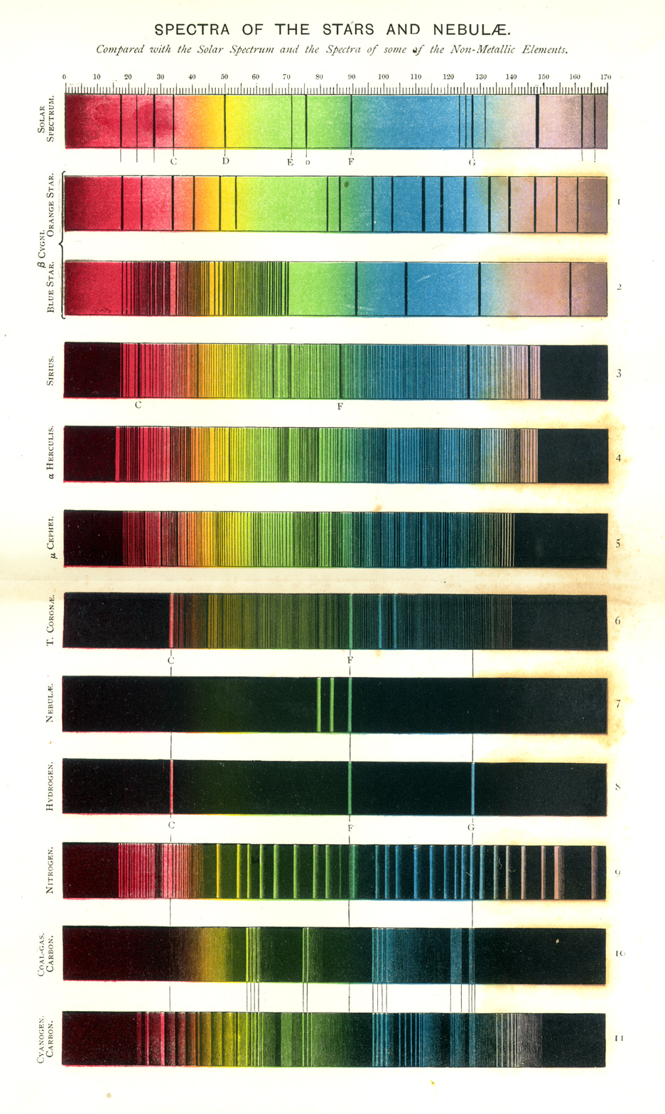
Figure 9 is a chromolithograph from Lockyer’s book (5), illustrating both absorption and emission (radiation) spectra. Spectrum 1 is the continuous spectrum, for reference. Spectra 2 through 8 are emission spectra: 2 is of sodium—note the doublet around 589 nm; 3 is of magnesium; 4 is from a salt of strontium; 5 and 6 are both of hydrogen, but at different pressures; 7 and 8, respectively, are from a nebula and the sun’s chromosphere. Spectra 9 and 10 are absorption spectra: 9 represents the absorption in the solar spectrum, and 10 represents the absorption of sodium vapor in the laboratory. Compare spectra 9 (emission) and 10 (absorption); both sodium. Lockyer began his career as an amateur astronomer in 1859 with Bunsen and Kirchhoff’s discoveries. He attached a spectroscope to his 6-1/4;” refracting telescope, and began observations that led to his appointment in 1875 as director of the Solar Physics Observatory at South Kensington. Interestingly, Lockyer was the founder of Nature, the scientific journal, which began in 1869, and which Lockyer edited for the first 50 years of its existence.

FILTERS – THESE ARE FUN!

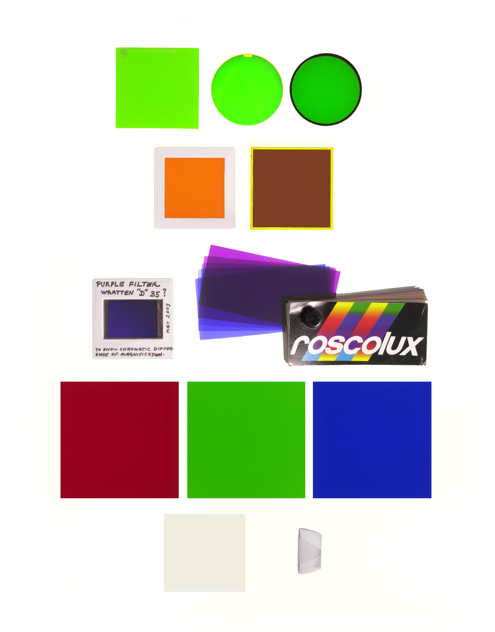
Figure 10 shows some of the filters that I used, including three greens—a Wratten No. 58, a GIF green interference filter, and a precision 546 nm interference filter; two oranges—a Roscolux No. 23 orange, and a precision 589 nm interference filter; a Wratten #35 (D) purple filter, and a combination of five Roscolux filters; the tricolor filters, Wratten #47, #61, and #29; and two examples of didymium glass, one a proper filter, and the other a scrap from the making of a wavelength standard.

Start, say, by putting a precision line Sodium D interference filter over your light-exit port (use a 10X-20X objective; condenser aperture diaphragm open). Look out to the left or right of the slit, and you will see an orange vertical line at 589 nm, with a width of about 10 nm. Now, substitute for the interference filter, a Rosco Roscolux #23 orange filter, and notice how much wider the bandpass is. This affords a dramatic demonstration as to why professional microscopists should use the more expensive precision line interference filters for refractive index determination, and why the much less expensive orange theatrical gel is more suited to student use in classrooms where economical large numbers of filters are required.

Another very informative experiment consists of comparing a Nilkon GIF green interference filter, and an Olympus 546 nm interference filter. The Olympus is very narrow in band width, and is ideal for Senarmont compensation; whereas, the other is much broader and more suited for use in phase contrast microscopy.

Didymium filters were very popular when used to make color film photomicrographs of H and E stained biomedical tissues. Today, the same didymium filters are still used to enhance the reds in H and E stained tissues, but now for digital imaging. Didymium is made up chiefly from a mixture of the rare earth oxides of neodymium and praseodymium, and has very strong and distinctive absorption bands. Place one of these filters anywhere in the light path, and note the very distinct dark absorption bands, the strongest being in the yellow where sodium lies. Glassblowers use eyeglasses made from didymium glass to filter out the yellow-colored flame due to sodium, so that they can watch the flow of the molten glass.

Didymium filters are made by Schott, and Corning, amongst others. At one time, didymium glass was sold by Nelson Gemmological Instruments (1 Lynhurst Road, Hampstead, London NW3 5PX, U.K. phone 020 7267 7199) as McCrone Wavelength Standard M-27.

Place various photographic filters in the light path, and notice the regions in which they absorb. More specifically, place Wratten filters #47 blue, #61 green, and #29 red in the light path, and notice how each one covers a different third of the spectrum. These three filters, known as the tricolor filters, are used in color separation work. Another combination is Wratten filters #47B, #58, and #25.

Peter Evennett has written a wonderful article (7) on adapting a consumer digital camera for photomicrography, in which he discusses and illustrates avoidance of chromatic difference of magnification. His illustrations involve the use of a purple filter to demonstrate blue and red images on either side of stage micrometer graduations in mis-matched objective/optical camera coupler systems. The filter he uses is a now- discontinued Wratten #35 (D) filter, formerly sold as part of a Kodak Photomicrography Filter Set.

I tried to duplicate the effects of this discontinued filter by combining Roscoe Roscolux filters. I noted the complete absence of the yellow/orange/green region in the #35 filter; only moderately wide red and blue bands. I started combining various Roscoe filters until I obtained a similar appearance in the resulting spectrum; maybe somewhat better than the #35. The combination of the following Roscoe filters is equivalent to the #35(D): #49 Medium Purple; #52 Light Lavender; #56 Gypsy Lavender; #349 Fisher Fuchsia; and either #355 Pale Violet, or #357 Royal Lavender.

Incidentally, by covering only the lower half of your light-exit port with your test filter, you will see both the absorption spectrum of the test filter, and the continuous spectrum for reference.

Solids, and particularly colored minerals, have been extensively studied with the microspectroscope. There is a 1915 Smithsonian publication by Wherry (8) that deals exclusively with the microspectroscope in mineralogy. Edgar T. Wherry, Assistant Curator, Division of Mineralogy and Petrology, U.S. National Museum, used a Crouch binocular microscope stand, fitted with a 37 mm focal length objective, and an Abbe-Zeiss “Spectral-Ocular” in the right-hand tube to make a survey of scores of colored minerals, including the rare earth minerals, the uranium minerals, and the garnet group. The results of the examination of about 200 minerals with the microspectroscope are presented in tabular form; groupings are by color (yellow or brown; red, pink or orange; blue; green; etc.). The absorption bands are recorded numerically under the general columns red, orange, yellow, green, blue, violet.

Colored liquids may also be viewed. These are best looked at by placing the colored liquid in a watchglass; that way, the effect of thickness of the liquid layer may be demonstrated. There are characteristic absorption spectra for a host of substances, including indigo, ammoniacal copper sulfate, tincture of chlorophyll, potassium dichromate, potassium permanganate, cobalt cyanide, didymium nitrate, cobalt chloride, and blood. This last item, blood, is of particular interest to me, because I used my simple microspectroscopic eyepiece in what turned out to be, at that time, the longest murder trial in the history of one of our northern states. But let me tell you this story as part of the background as to why I made the microspectroscopic eyepiece in the first place.

BACKGROUND AND HISTORY OF THE MICROSPECTROSCOPE

When I first joined McCrone Associates about 40 years ago, I was delighted to discover in the library a complete run of both the Journal of the Royal Microscopical Society, and the Journal of the Quekett Microscopical Club. I resolved to read both…and I did…it took me eight years! Along the way, I left little bits of paper in each volume noting special topics. For me, one of the most fascinating topics was the invention of the microspectroscope in the 1860s.

Wollaston in 1802 and Fraunhofer in 1814 independently discovered the fine black lines in the spectrum of sunlight; and Kirchhoff in 1859 introduced spectrum analysis. The spectroscope as a refined analytical instrument was first made known by Kirchhoff and Bunsen in 1860. It was F. Hoppe who first described the absorption bands of human blood in 1862. Browning and Huggins constructed the first microspectroscope, but Sorby, the founder of petrography and metallography, almost immediately suggested improvements in the prism design. The “Sorby-Browning Micro-spectroscopic Eye-piece” (Figures 4 and 5) was constructed, and used to investigate many materials. You can read about these early designs of the microspectroscope in Hogg’s The Microscope, Its History, Construction, and Application (9).

From 1865 to 1871, there were a series of articles published by Sorby and Browning (10) on the applications of the microspectroscope, and the detection of blood was discussed in all. Several points stuck with me, including the fact that the absorption spectrum of blood changes with age. Sorby published the absorption spectra of human blood under different conditions (11, 12, 13). What impressed me most was that by employing a high magnification objective, the absorption spectrum of human blood was obtained from a single red blood cell.

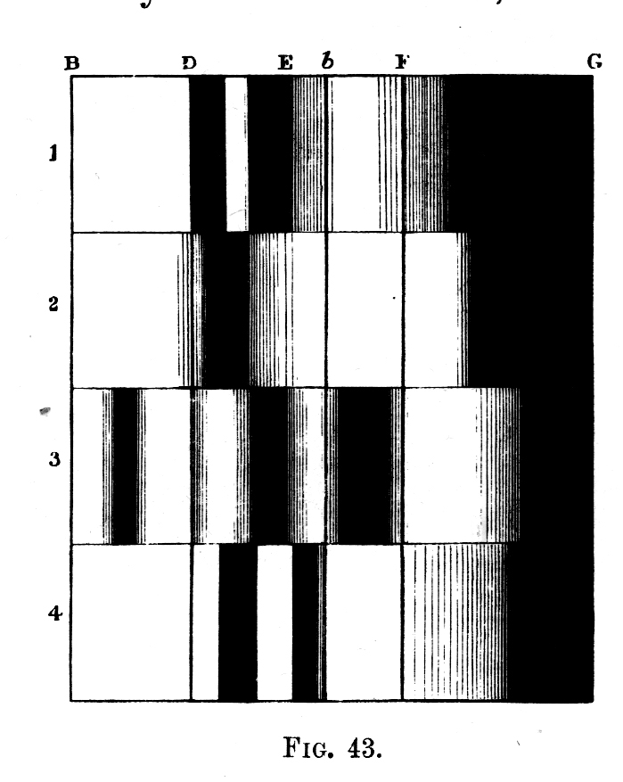
Professor Stokes also examined the subject of oxidized and deoxidized blood, and published a paper on his findings in the Proceedings of the Royal Society in 1864. Stokes’ diagram of the absorption bands of blood were included in Roscoe’s book (4), and is presented here as Figure 11. Oxidized and deoxidized blood absorption bands are shown in the first and second spectra; and after converting to haematin by the action of acid, the absorption spectra change, but show similar differences for oxidized (third spectrum) and deoxidized (fourth spectrum) states. Stokes’ diagram of the absorption bands of blood are also included in Schellen’s book (6).

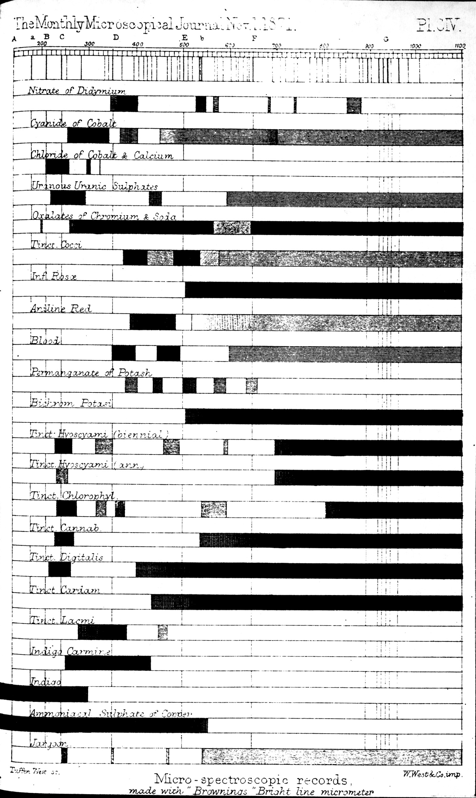
The absorption spectrum of blood, as well as other interesting substances, is also recorded in a woodcut published in The Monthly Microscopical Journal for November 1871 (14), and is shown here as Figure 12.

I made the simple microspectroscopic eyepiece to play with; I wanted to see for myself these things that had been described a hundred years earlier. Just as I had finished assembling the microspectroscopic eyepiece, fortune favored me by way of an accident to one of my colleagues. Robert Z. Muggli, staff chemist and Associate at McCrone Associates, cut himself while breaking glass tubing in the wet lab. Several of us were present, and everyone ran for first-aid supplies, except me; I ran for microscope slides, and managed to collect enough blood for my studies before the others returned. Bob was good-natured about it when he learned that I intended to record the changes in the absorption spectrum of his blood over time. [Sorby had no trouble in detecting 50 year old blood.]

Shortly thereafter, as fate would have it, I was hired by the defense for a case in which the accused was charged with the kidnap, rape, and murder of a teen-aged girl in one of our northern states. There was a great deal of physical evidence in the case, but the relevant sample concerned a small, reddish-brown deposit taken by the State from the dashboard of the accused’s truck; he is said to have taken the girl into his truck after first striking the back of the motorscooter she was riding on, knocking her off. The reddish-brown deposit was thought to be blood. The State was reluctant to conduct tests for typing because of the small amount present. The defense attorney said that he needed to know if the reddish-brown deposit was blood or not; if it was, the accused would have to account for it; if it was not, precious time could be devoted to the many other items of physical evidence. The defense attorney asked me if I could tell if the spot was blood just by looking at it with my microscope. I said “yes,” and the next day, above the protests of the Crime Lab personnel and warnings that I could not conduct any chemical or other destructive tests, and with my repeated assurances that I was only going to look at the material, I was allowed to put the sample on the stage of my portable microscope. I inserted the microspectroscopic eyepiece, which, of course, you could not tell from any other eyepiece from the outside, and tilted my mirror to the overhead laboratory lights, which were fluorescent. Having now my marker wavelengths from the superimposed mercury lines, I looked for the absorption bands around 400-450 nm, 535-550 nm, 575-585 nm, 730+ nm, and did not see them. I thanked them, returned the sample, and left. I told the attorney I did not know what the reddish-brown deposit was, but it was not blood. The State never introduced the deposit into evidence.

It was a source of enormous personal satisfaction to have been able to use my simple microspectroscopic eyepiece, which cost about 25¢ to make, to help make a decision on such an important question. As a matter of curiosity, I searched the then-current textbooks of criminalistics, and never did find this method of blood detection mentioned. I guess it got lost somewhere over the last 140 years.

The microspectroscopic examination of blood is, however, thoroughly discussed in at least one book on medical jurisprudence and toxicology; the twelfth edition of Glaister and Rentoul’s Medical Jurisprudence and Toxicology (15) contains a complete description of the method together with reference absorption spectra for blood.

Anyway, for a few dollars, and an hour or two of your time, I guarantee you will learn something about filters and colored solid and liquid specimens that you didn’t know before—and have fun doing it—by constructing and using your simple microspectroscopic eyepiece.

REFERENCES

(1) Delly, John Gustav (1966). “A Simple Microspectroscopic Ocular”. The Microscope 15 (4), pp. 143-144.

(2) Needham, George Herbert (1958). The Practical Use of the Microscope. Charles C. Thomas, Springfield, Illinois. The Microspectroscope is discussed on pp. 265-267.

(3) Delly, John Gustav (1991). “Conversion of Olympus Polarizing Condenser to Non-Pol”. The Microscope 39, pp. 127-130.

(4) Roscoe, Henry E. (1869). Spectrum Analysis: Six Lectures Delivered in 1868 Before the Society of Apothecaries of London. Macmillan, London.

(5) Lockyer, J. Norman (1878). Studies in Spectrum Analysis. Kegan Paul, London.

(6) Schellen, H. (1872). Spectrum Analysis (translated from the Second Enlarged Revised German edition). Longmans, London.

(7) Evennett, Peter (2000). “The New Photomicrography”. Proceedings of the Royal Microscopical Society. 35, pp. 253-256.

(8) Wherry, Edgar T. (1915). “The Microspectroscope in Mineralogy”. Smithsonian Miscellaneous Collections, Volume 65, Number 5, Publication 2362, Smithsonian Institution, Washington, D.C.

(9) Hogg, Jabez (1898). The Microscope; Its History, Construction, and Application. George Routledge & Sons Ltd., London.

(10) Browning, John (1865). “On the Application of the Spectroscope to the Microscope”. Transactions of the Microscopical Society of London. XIII, pp. 107-113.

(11) Sorby, Henry C. (1865). “On the Application of Spectrum – Analysis to Microscopical Investigations, and Especially to the Detection of Blood-Stains”. The Quarterly Journal of Science. Volume II. Pp. 198-215.

(12) Sorby, Henry C. (1871). “On Some Improvements in the Spectrum Method of Detecting Blood”. The Monthly Microscopical Journal: Transactions of the Royal Microscopical Society. Volume VI. Pp. 9-17.

(13) Sorby, Henry C. (1871). “On the Examination of Mixed Colouring Matters with the Spectrum Microscope” . The Monthly Microscopical Journal: Transactions of the Royal Microscopical Society. Volume VI. Pp.124-134.

(14) Bridge, H.G. (1871). “Mapping with the Micro-spectroscope, withthe Bright-line Micrometer”. The Monthly Microscopical Journal: Transactions of the Royal Microscopical Society. Volume VI. Pp. 224-225.

(15) Glaister, John and Edgar Rentoul (1966). Medical Jurisprudence and Toxicology. Livingstone, Edinburgh and London.